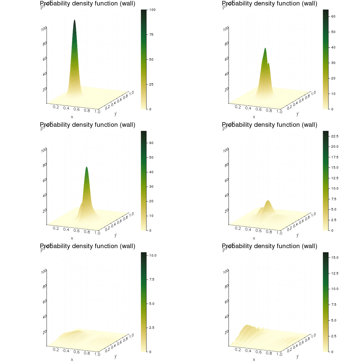
Now we are taking the previous 1 dimensional equations and making them two dimensional. The following is the code used to do this.
using Plots
include("Imag.jl")
include("Imag_2D.jl")
include("Real_2D.jl")

ENV["PLOTS_TEST"] = "true"
ENV["GKSwstype"] = "100"
N = 200
x_0 = fill(0.25, (N,N))
y_0 = fill(0.5, (N,N))
C = fill(10.0, (N,N))
sigma_squared = fill(0.01, (N,N))
k_0 = 40.0
delta_x = 1/200
delta_t = 0.00001
a = range(0, stop = 1, length = N)
x = zeros(N,N)
for i = 1:N
   for j = 1:N
      x[i,j] = a[j]
   end
end
y = zeros(N,N)
for i = 1:N
   for j = 1:N
      y[j,i] = a[j]
   end
end
V = zeros(N,N)
for i = 1:N
   for j = convert(Int64, N/2):N
      V[i,j] = 1e3
   end
end
# Create a 2D potential wall
# V=zeros(N,N)
# V(:, 100:200)=1e3
psi_stationary = C.*exp.((-(x-x_0).^2)./sigma_squared).*exp.((-(y-y_0).^2)./sigma_squared)
plane_wave = exp.(1im*k_0*x) #+1im*k_0*y)
psi_z = psi_stationary.*plane_wave
R_initial = real(psi_z)
I_initial = imag(psi_z)
I_current = I_initial
R_current = R_initial
I_next = imag_psi(N, I_current, R_current, delta_t, delta_x, V)

anim = @animate for time_step = 1:2000
   global R_current, I_current, N, delta_t, delta_x, V, prob_density
   R_next = real_psi_2D(N, R_current, I_current, delta_t, delta_x, V)
   R_current = R_next
   I_next = imag_psi_2D(N, I_current, R_current, delta_t, delta_x, V)
   prob_density = R_current.^2 + I_next.*I_current
   I_current = I_next
   surface(x[1,:],y[:,1], prob_density,
      title = "Probability density function (wall)",
      xlabel = "x",
      ylabel = "y",
      zlabel = "ps*psi",
      xlims = (0,1), ylims = (0,1), zlims = (0,100),
      color = :speed,
      axis = true,
      grid = true,
      cbar = true,
      legend = false,
      show = false
   );
end every 5
gif(anim, "./Figures/bigtwoD_Leapfrog_wall.gif", fps=30)
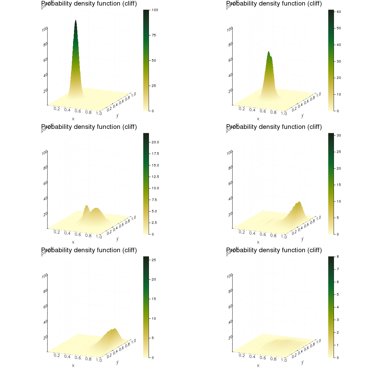
And this is the results of the wave hitting a wall and a cliff

