Since there is no monitor attached to the cluster an error will occur when Julia looks to find a display to output the graph to. To fix this error we must tell Julia to not output to any display. This is done by adding the following two lines at the beginning of the program.

ENV["PLOTS_TEST"] = "true"
ENV["GKSwstype"] = "100"

Now we are taking the previous 1 dimensional equations and making them two dimensional. The following is the code used to do this.

using Plots
include("Imag.jl")
include("Imag_2D.jl")
include("Real_2D.jl")

ENV["PLOTS_TEST"] = "true"
ENV["GKSwstype"] = "100"
N = 200
x_0 = fill(0.25, (N,N))
y_0 = fill(0.5, (N,N))
C = fill(10.0, (N,N))
sigma_squared = fill(0.01, (N,N))
k_0 = 40.0
delta_x = 1/200
delta_t = 0.00001
a = range(0, stop = 1, length = N)
x = zeros(N,N)
for i = 1:N
   for j = 1:N
      x[i,j] = a[j]
   end
end
y = zeros(N,N)
for i = 1:N
   for j = 1:N
      y[j,i] = a[j]
   end
end
V = zeros(N,N)
for i = 1:N
   for j = convert(Int64, N/2):N
      V[i,j] = 1e3
   end
end
# Create a 2D potential wall
# V=zeros(N,N)
# V(:, 100:200)=1e3
psi_stationary = C.*exp.((-(x-x_0).^2)./sigma_squared).*exp.((-(y-y_0).^2)./sigma_squared)
plane_wave = exp.(1im*k_0*x) #+1im*k_0*y)
psi_z = psi_stationary.*plane_wave
R_initial = real(psi_z)
I_initial = imag(psi_z)
I_current = I_initial
R_current = R_initial
I_next = imag_psi(N, I_current, R_current, delta_t, delta_x, V)

anim = @animate for time_step = 1:2000
   global R_current, I_current, N, delta_t, delta_x, V, prob_density
   R_next = real_psi_2D(N, R_current, I_current, delta_t, delta_x, V)
   R_current = R_next
   I_next = imag_psi_2D(N, I_current, R_current, delta_t, delta_x, V)
   prob_density = R_current.^2 + I_next.*I_current
   I_current = I_next
   surface(x[1,:],y[:,1], prob_density,
      title = "Probability density function (wall)",
      xlabel = "x",
      ylabel = "y",
      zlabel = "ps*psi",
      xlims = (0,1), ylims = (0,1), zlims = (0,100),
      color = :speed,
      axis = true,
      grid = true,
      cbar = true,
      legend = false,
      show = false
   );
end every 5
gif(anim, "./Figures/bigtwoD_Leapfrog_wall.gif", fps=30)

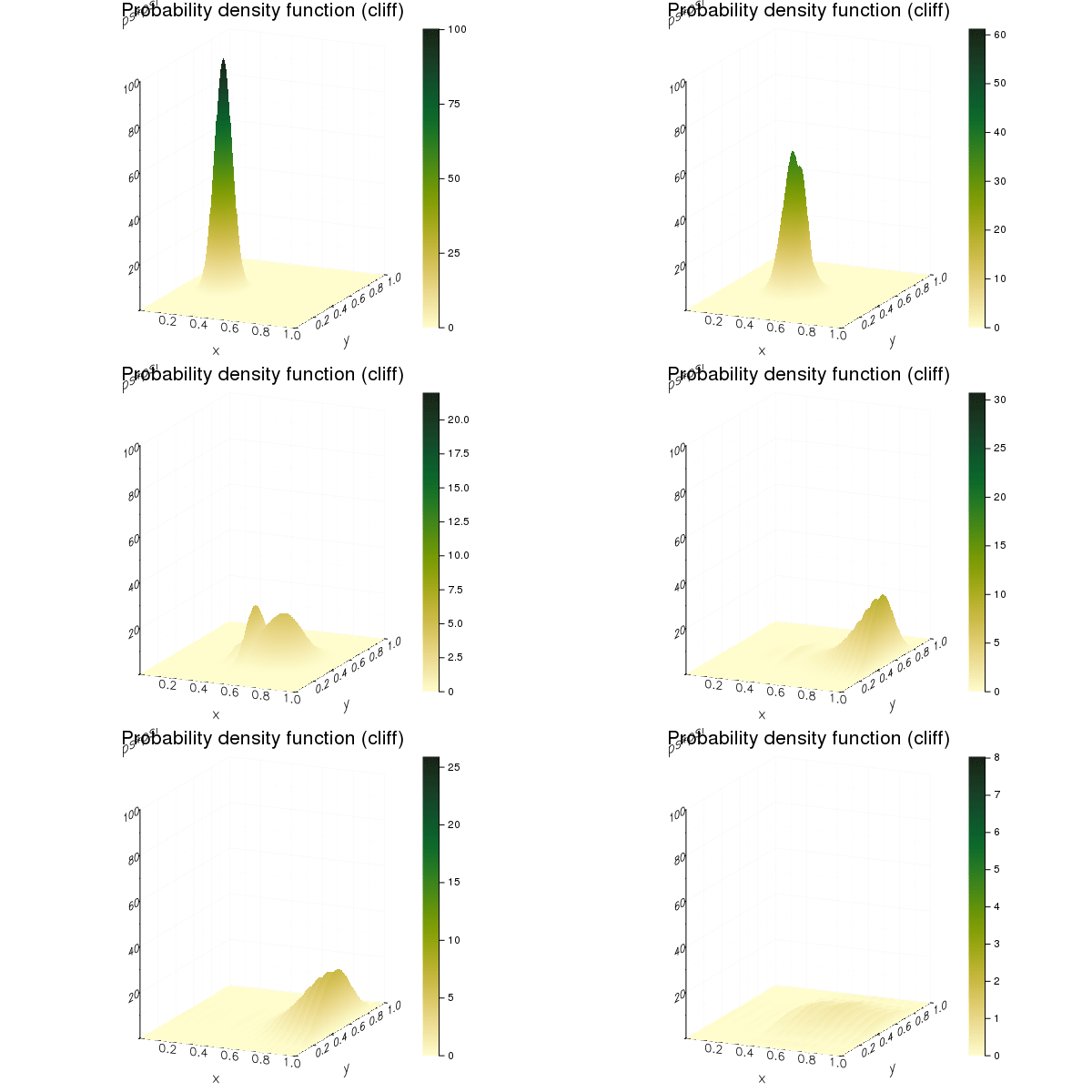
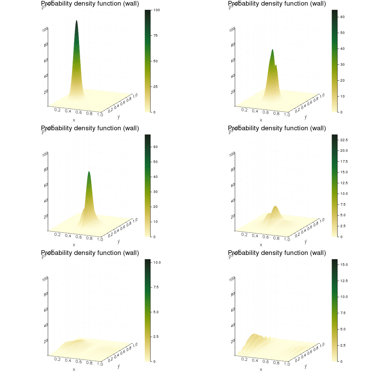
And this is the results of the wave hitting a wall and a cliff

The leapfrog method is a method that enables us to calculate a wave in motion over time. It does this by calculating the wave equations real and imaginary components in sequential order then adding the results to form the wave over time.

using Plots
include("Real.jl")
include("Imag.jl")
function leapfrog()
   ENV["PLOTS_TEST"] = "true"
   ENV["GKSwstype"] = "100"
   N = 1000
   x = collect(0:(1/(N-1)):1)
   x_0 = fill(0.4, N)
   C = fill(10.0, N)
   σ_sqrd = fill(1e-3, N)
   k_0 = 500.0
   Δ_x = 1e-3
   Δ_t = 5e-8
   ψ = C.*exp.((-(x-x_0).^2)./σ_sqrd).*exp.((k_0*x)*1im)
   R_cur = real(ψ)
   I_cur = imag(ψ)
   V = fill(0.0, N)
   for i = 600:N
      V[i] = -1e6
   end
   I_next = imag_psi(N, I_cur, R_cur, Δ_t, Δ_x, V)
   # Do the leapfrog
   anim = @animate for time_step = 1:15000
      #global R_cur, I_cur
      R_next = real_psi(N, R_cur, I_cur, Δ_t, Δ_x, V)
      R_cur = R_next
      I_next = imag_psi(N, I_cur, R_cur, Δ_t, Δ_x, V)
      prob_density = R_cur.^2+I_next.*I_cur
      I_cur = I_next
      plot(x, prob_density,
      title = "Reflection from cliff",
      xlabel = "x",
      ylabel = "Probability density",
      ylims = (0,200),
      legend = false,
      show = false
      )
      plot!(x,abs.(V))
   end every 10
   gif(anim, "./Figures/ExtraLeapFrogCliff.gif", fps=30)
   return 0
end

@time leapfrog()

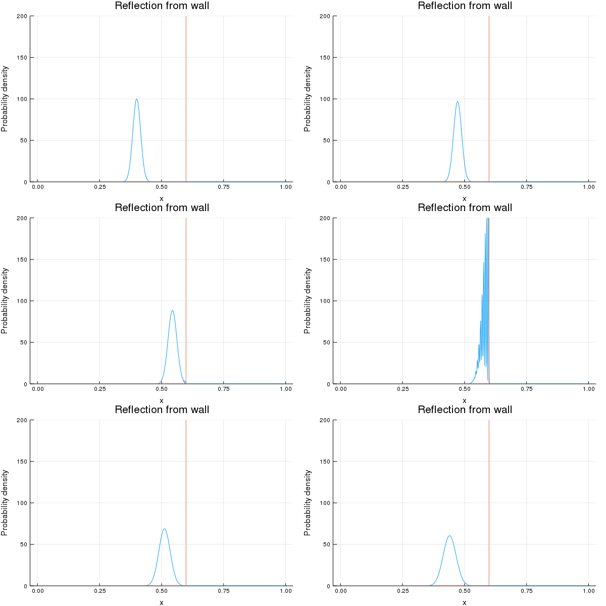
This code can be used to produce the affect of a wave hitting a wall and a cliff or any other barrier/obstacle. The following two graphs are the results of the wave hitting a wall and a cliff.

To view the code used to create these the following plots please visit my github at: https://github.com/Tim-Mer/Julia_Beowulf

Using this equation with the initial constraints of:

• x = 0.0005
• x_0 = 0.4
• C = 25
• sigma_squared = 1e-3
• delta_x = 0.0005
• delta_t = 0.2
• k_0 = 500

the following graphs were created.

Step 1. Install Ubuntu on all the nodes in the cluster. As using Linux is the easiest way to set up a Beowulf Cluster.

Step 2. Make sure everything is up to date using the following commands in terminal

sudo apt update sudo apt upgrade -y

Step 3. Is to install all the required packages onto the cluster. This is done with the following command.

sudo apt install nfs-common ssh mpi build-essential libatomic1 python gfortran perl wget m4 cmake pkg-config -y

Step 4. Edit the host file of all the nodes so that they can all communicate. An example host file is shown below

Open using: sudo nano /etc/hosts

File:
 127.0.0.1 localhost
 192.168.1.10 masternode
 192.168.1.11 node1
 192.168.1.12 node2
 192.168.1.13 node3

Step 5. Create the user account that will be used by the cluster to communicate. Do not use the root account for this. The account can be created using the following command.

sudo adduser Juser --uid 999

Make sure to create an account with the same name on all the nodes in the cluster. A uid of less than 1000 is used so that the user does not show up on the login screen.

Step 6. On the master node you need to add the following steps.

Step 6.1. Use the following commands in terminal to set up the shared drive space.

Install the nfs kernel server using the following command

sudo apt install nfs-kernel-server -y

ls -l /home/ | grep Juser

If you are not using the Juser home directory, make sure the Juser own it by running the following command

sudo chown Juser:Juser /path/to/dir

Open the /etc/exports file and add the following line

/Juser/home *(rw,sync,no_subtree_check)

Run,

sudo service nfs-kernel-server restart
sudo exportfs -a

to restart the nfs server and share the drive location on the network. To ensure that the nodes located on the network can access the location add the following exception to the ufw.

sudo ufw allow from 192.168.1.0/24

This is done assuming you have used the same network and have set up the nodes using a static ip.

Step 6.2. Setting up ssh. This is still being done from the master node.

Run the following commands to generate ssh keys and copy them into the shared directory so that all nodes can access each other using the same key. Do not add a password when asked to create one. Just hit enter. This means that the nodes will have password-less ssh access to each other.

su Juser<br>ssh-keygen
ssh-copy-id localhost

Step 7. On all the other nodes you now need to mount the shared drive location. This is done using the following command.

sudo mount masternode:/home/Juser /home/Juser

To make sure that the location is mounted at startup, add the following line to the /etc/fstab file.

masternode:/home/Juser /home/Juser nfs

Step 8. Restart all the nodes and make sure they can all access the shared drive location and that you can ssh between all the nodes without entering a password.

Step 9. To install Julia, download the official binaries from their website and export the downloaded file to your home directory.

To enable running Julia without having to cd into the directory you can link the location of the binary to any of the directories labeled on your $PATH. This can be done using the following command.

sudo ln -s /path/to/Julia(version)/bin/Julia /usr/local/bin/

In this case the full location was

sudo ln -s /home/Juser/Julia-1.1.0/bin/Julia /usr/local/bin/

You should now be able to run Julia by typing Julia in the terminal window.

I have begun to learn the Julia programming language and as always the first program I wrote displays the text “Hello World”

I am going to use the Atom IDE with the “uber-Juno” package installed which allows the easy writing of scripts using the Julia programming language.

I have put together a short video where I test that all computers are in working condition.

I was talking to one of the lab technicians today and he has built a CUDA rig with dual Nvidia 1060’s which together have 2560 CUDA cores. These core can be used as hardware acceleration for problems such as the quantum confinement problem.

Using this rig and the Julia programming language it may be possible to use hardware acceleration and compare its performance to the Beowulf cluster.

A Beowulf Cluster is usually a cluster of ordinary computers which have been connected over a LAN network. This can be done easily using a switch and some Ethernet cables. Together these computers computational power will be combined to solve computationally intensive tasks such as protein folding.

A Beowulf Cluster is usually run using a Unix based operating such as Ubuntu.

A basic Beowulf Cluster is composed of one server node, which is seen as the base computer and is the access point to all other nodes in the cluster. All other nodes are called client nodes and they are used as the backbone of the system, providing the required computational power.

The nodes communicate using Message Passing Interface (MPI) and Parallel Virtual Machine (MPV)

My name is Timothy Merriman, and I will be undertaking a project under the following title: Construction of a Beowulf High Performance Computing Cluster for simulation of quantum confinement.

I am undertaking this project as part of my final year in Technological University Dublin (Dublin Institute of Technology) DT021A. This blog will be used to document my progress.